Introduction to Quantum Computing

• Used to describe quantum states: let \(a, b \in \mathbb{C}^2\) (2 dimensional vector with complex entries)
  • ket: \(| a \rangle = \begin{pmatrix} a_0 \\ a_1 \end{pmatrix}\)
  • bra: \(\langle b | = | b \rangle^{\dagger} = (b_0^*, b_1^*)\)
  • bra-ket: \(\langle b | a \rangle = a_0 b_0^* + a_1 b_1^* = \langle a | b \rangle^*\)
  • ket-bra: \(| a \rangle \langle b| = \begin{pmatrix} a_0 b_0^* & a_0 b_1^* \\ a_1 b_0^* & a_1 b_1^* \end{pmatrix}\)

• We define the pure states \(| 0 \rangle = \begin{pmatrix} 1 \\ 0 \end{pmatrix}\) and \(| 1 \rangle = \begin{pmatrix} 0 \\ 1 \end{pmatrix}\) which are orthogonal \(\langle 0 | 1 \rangle = 1 . 0 + 0 . 1 = 0\)

  • \(|0\rangle \langle 0| = \begin{pmatrix} 1 & 0 \\ 0 & 0 \end{pmatrix}\)
  • \(|1\rangle \langle 1| = \begin{pmatrix} 0 & 0 \\ 0 & 1 \end{pmatrix}\)

  -\(\rho=\begin{pmatrix} \rho_{00} & \rho_{01} \\ \rho_{10} & \rho_{11} \end{pmatrix}=\rho_{00} |0\rangle \langle 0| + \rho_{01} |0\rangle \langle 1| + \rho_{10} |1\rangle \langle 0| + \rho_{00} |1\rangle \langle 1|\)

• All quantum states can be described by density matrices, ie normalized positive Hermitian operators, \(\rho\) with \(tr(\rho)=1\), \(\rho\geq 0\), \(\rho=\rho^{\dagger}\)

  for \(\rho=\begin{pmatrix} \rho_{00} & \rho_{01} \\ \rho_{10} & \rho_{11} \end{pmatrix}\), \(tr(\rho)=\rho_{00}+\rho_{11}=1\), \(\langle \psi | \rho | \psi \rangle \geq 0 \quad \forall \psi\),

• All quantum states are normalized, ie, \(\langle \psi | \psi \rangle = 1\)
• Spectral decomposition: for every density matrix \(\rho \exists\) and orthonormal basis \(\{\ i \rangle\}_i\) s.t. \(\rho = \sum_i \lambda_i | i \rangle \langle i |\) where \(| i \rangle\) eigenstates, \(\lambda_i\) eigenvalues and \(\sum_i \lambda_i = 1\)
• A density matrix is pure if \(\rho = | \phi \rangle \langle \phi |\), otherwise it is mixed.
  • if \(\rho\) is pure, one eigenvalue equals 1, all others are 0. \(tr(\rho^2)=\sum_i \lambda_i^2=1\) if \(\rho\) pure, otherwise \(tr(\rho^2)<1\)

We choose orthogonal bases to describe & measure quantum states (projective measurement). During a measure onto the basis\(\{ | 0 \rangle , | 1 \rangle \}\), the state will collapse into either state \(| 0 \rangle\) or \(| 1 \rangle\). We call this a z-measurement (\(| 0 \rangle\) and \(| 1 \rangle\) are the eigenstates of \(\sigma_z\))

There are infinitely many different bases, but the most common ones are: \(\{ | + \rangle, | - \rangle \} = \{ \frac{1}{\sqrt{2}} (| 0 \rangle + | 1 \rangle), \frac{1}{\sqrt{2}} (| 0 \rangle - | 1 \rangle) \}\) (eigenstates of \(\sigma_x\)) \(\{ | +i \rangle, | -i \rangle \} = \{ \frac{1}{\sqrt{2}} (| 0 \rangle + i | 1 \rangle), \frac{1}{\sqrt{2}} (| 0 \rangle - i | 1 \rangle) \}\) (eigenstates of \(\sigma_y\))

• Born Rule: the probability that a state \(| \psi \rangle\) collapses during a projective measurement onto the basis \(\{ |X \rangle, |X^\perp \rangle \}\) to the state \(| X \rangle\) is given by \(P(x) = | \langle x | \psi \rangle|^2\) where \(\sum_i P(x_i) = 1\)

We can write any normalized (pure) state as \(| \psi \rangle = \cos{\frac{\theta}{2}} | 0 \rangle + e^{i \phi}\sin{\frac{\theta}{2}} | 1 \rangle\) where \(\phi \in [0, 2 \pi ]\) describes the relative phase and \(\theta \in [0, \pi]\) determines the probability to measure \(| 0 \rangle\) and \(| 1 \rangle\): \(P(| 0 \rangle) =\cos^2 \frac{\theta}{2}\) and \(P(| 1 \rangle)=\sin^2 \frac{\theta}{2}\)

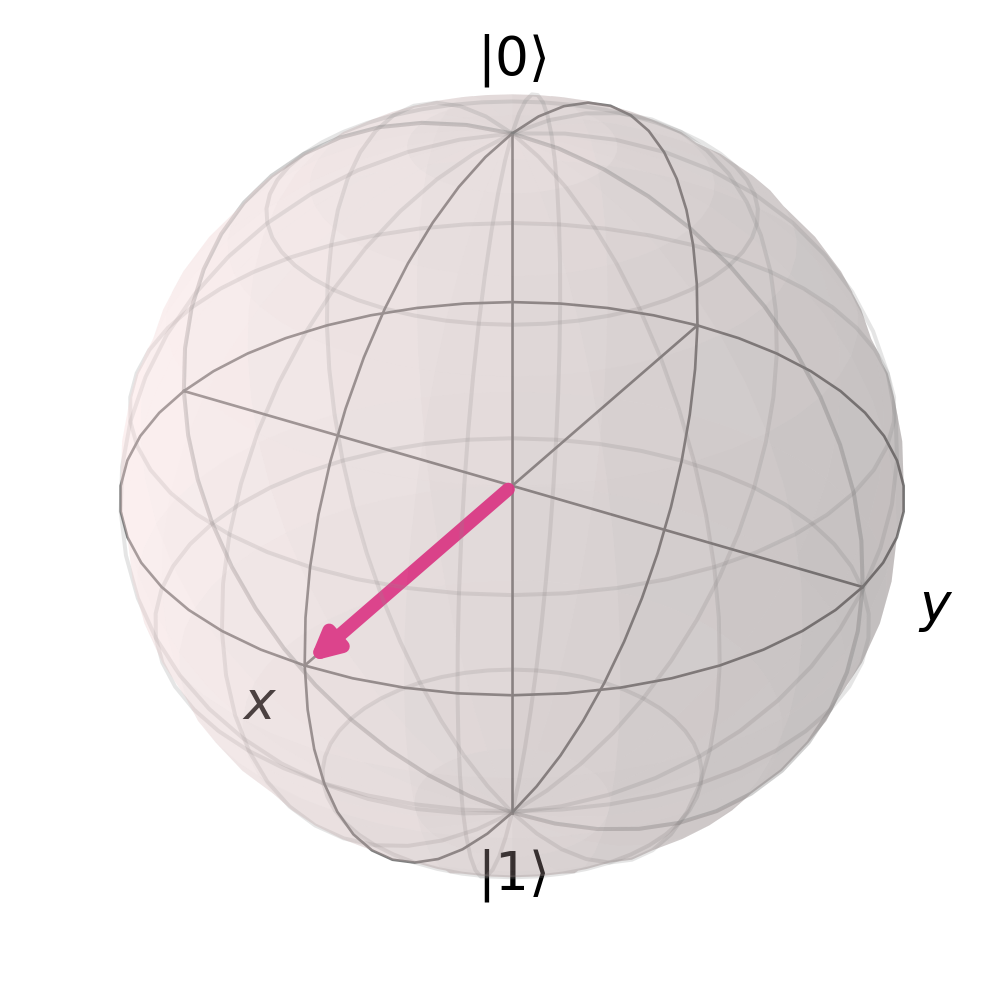
All normalized pure states can be illustrated on the surface of a sphere with radius 1, which we call the Bloch sphere. The coordinates of such a state are given by the Bloch vector \(\vec{r} =\begin{pmatrix} \sin{\theta} \cos{\phi} \\ \sin{\theta} \sin{\phi} \\ \cos{\theta}\end{pmatrix}\)

On the Bloch sphere, angles are twice as big as in Hilbert space. Here, \(\theta\) is the angle on the sphere while \(\frac{\theta}{2}\) is the actual angle in Hilbert space.

• Classical example: the NOT gate (add scheme)
• Quantum example: as quantum theory is unitary, quantum gates are represented by unitary matrices: \(\mathcal{U}^{\dagger}\mathcal{U}=1\)

We use tensor products to describe multiple states

\(| a \rangle \otimes | b \rangle = \begin{pmatrix} a_1 \\ a_2 \end{pmatrix} \otimes \begin{pmatrix} b_1 \\ b_2 \end{pmatrix} = \begin{pmatrix} a_1 b_1\\ a_1 b_2 \\ a_2 b_1 \\ a_2 b_2 \end{pmatrix}\)

Example: system A is in state \(| 1 \rangle_A\) and system B is in state \(| 0 \rangle_B\)

the total bipartite state is \(| 10 \rangle_{AB} = | 1 \rangle_A \otimes | 0 \rangle_B = \begin{pmatrix} 0 \\ 1 \end{pmatrix} \otimes \begin{pmatrix} 1 \\ 0 \end{pmatrix} = \begin{pmatrix} 0 \\ 0 \\ 1 \\ 0 \end{pmatrix}\)

States of this form are called uncorrelated, but there are also bipartite states that cannot be written as \(| \psi \rangle_A \otimes | \phi \rangle_B\).

These states are correlated and sometimes even entangled (very strong correlation)

e.g. \(| \psi^{(00)}\rangle_{AB}= \frac{1}{\sqrt{2}} (| 00 \rangle_{AB} + | 11 \rangle_{AB}) = \frac{1}{\sqrt{2}} \begin{pmatrix} 1 \\ 0 \\ 0 \\ 1 \end{pmatrix}\) a so-called Bell state, used for teleportation, cryptography, Bell test, …

Classical example: XOR gate (add scheme) irreversible: given the output we cannot recover the input

XOR	input	output
	x y	x + y
	0 0	0
	0 1	1
	1 0	1
	1 1	0

Quantum example: CNOT gate (add circuit)

as quantum theory is unitary, gates are reversible

\(\text{CNOT}=\begin{pmatrix} 1 & 0 & 0 & 0 \\ 0 & 1 & 0 & 0 \\ 0 & 0 & 0 & 1 \\ 0 & 0 & 1 & 0 \end{pmatrix}\)

\(\text{CNOT} | 00 \rangle_{xy} = | 00 \rangle_{xy}\)

\(\text{CNOT} | 10 \rangle_{xy} = | 11 \rangle_{xy}\)

We can show that every classical function \(f\) can be described by a reversible circuit.

Quantum circuits can perform all functions that can be calculated classically.

There are four so-called Bell states that are maximally entangled and constitute an orthonormal basis:

\(| \psi^{00}\rangle = \frac{1}{\sqrt{2}} (| 00 \rangle + | 11 \rangle)\)

\(| \psi^{10}\rangle = \frac{1}{\sqrt{2}} (| 00 \rangle - | 11 \rangle)\)

\(| \psi^{01}\rangle = \frac{1}{\sqrt{2}} (| 01 \rangle + | 10 \rangle)\)

In general, we can write \(| \psi^{ij}\rangle = ( \mathcal{1} \otimes \sigma_x^j \sigma_z^i) | \psi^{00} \rangle\)

(add scheme)

\(\mid ij \rangle_{AB}\)		\(\mathcal{H}_A \otimes \mathdd{1}_B \mid ij \rangle_{AB}\)		\(\mid \psi^{ij} \rangle\)
\(\mid 00 \rangle\)	\(\mathcal{H_A}\)	\(\frac{1}{\sqrt{2}}(\mid 00 \rangle + \mid 10 \rangle)\)	\(\text{CNOT}_{AB}\)	\(\frac{1}{\sqrt{2}}(\mid 00 \rangle + \mid 11 \rangle) = \mid \psi^{00}\rangle\)
\(\mid 01 \rangle\)		\(\frac{1}{\sqrt{2}}(\mid 01 \rangle + \mid 11 \rangle)\)		\(\frac{1}{\sqrt{2}}(\mid 01 \rangle + \mid 10 \rangle) = \mid \psi^{01}\rangle\)
\(\mid 10 \rangle\)		\(\frac{1}{\sqrt{2}}(\mid 00 \rangle + \mid 10 \rangle)\)		\(\frac{1}{\sqrt{2}}(\mid 00 \rangle - \mid 11 \rangle) = \mid \psi^{10}\rangle\)
\(\mid 11 \rangle\)		\(\frac{1}{\sqrt{2}}(\mid 01 \rangle - \mid 11 \rangle)\)		\(\frac{1}{\sqrt{2}}(\mid 01 \rangle - \mid 10 \rangle) = \mid \psi^{11}\rangle\)

(add scheme)

classical outcomes \(i,j\) correspond to a measure of the state \(| \psi^{ij} \rangle\)

Alice wants to send her (unknown) state \(|\phi \rangle_S = \alpha | 0 \rangle_S + \beta | 1 \rangle_S\) to Bob. She can only send him two classical bit though. They both share the maximally entangled state \(| \psi^{00} \rangle_{AB} = \frac{1}{\sqrt{2}} (| 00 \rangle_{AB} + | 11 \rangle_{AB} )\).

• Initial state of the total system:

\(| \phi \rangle_S \otimes | \psi^{00} \rangle_{AB}\)

• Protocol

(add scheme)

1. Alice performs a measurement on S and A in the Bell basis.
2. She sends her classical outputs \(i,j\) to Bob.
3. Bob applies \(\sigma_z^i \sigma_x^j\) to his qubit and gets \(| \phi \rangle\).

Alice’s meas.	Bob’s state	Alice sends	Bob applies	Bob’s final state
\(\mid \psi^{00}\rangle\)	\(\mid \phi \rangle_B\)	0 0	\(1\)	\(\mid \phi \rangle_B\)
\(\mid \psi^{01}\rangle\)	\(\sigma_x \mid \phi \rangle_B\)	0 1	\(\sigma_x\)	\(\mid \phi \rangle_B\)
\(\mid \psi^{10}\rangle\)	\(\sigma_z \mid \phi \rangle_B\)	1 0	\(\sigma_z\)	\(\mid \phi \rangle_B\)
\(\mid \psi^{11}\rangle\)	\(\sigma_x \sigma_z \mid \phi \rangle_B\)	1 1	\(\sigma_z \sigma_x\)	\(\mid \phi \rangle_B\)

Note that Alice’s state collapsed during the measurement, so she does not have the initial state \(| \phi \rangle\) anymore. This is expected due to the no-cloning theorem, as she cannot copy her state, but just send her state to Bob when destroying her own.